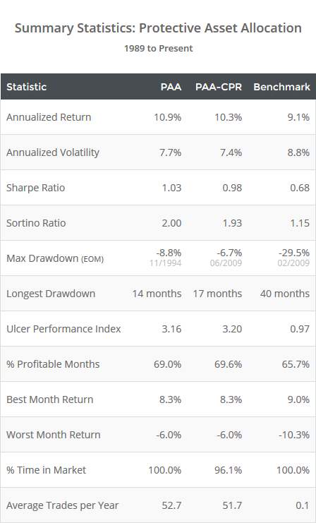
This is a test of two variations of the Protective Asset Allocation (PAA) strategy from Wouter Keller and JW Keuning’s paper: PAA: A Simple Momentum-based Alternative to Term Deposits. The strategy is notable for its aggressive use of a “crash protection” asset that has resulted in extremely low drawdowns relative to return. Results from 1989, net of transaction costs, follow.
Read more about our backtests or let AllocateSmartly help you follow this strategy in near real-time.
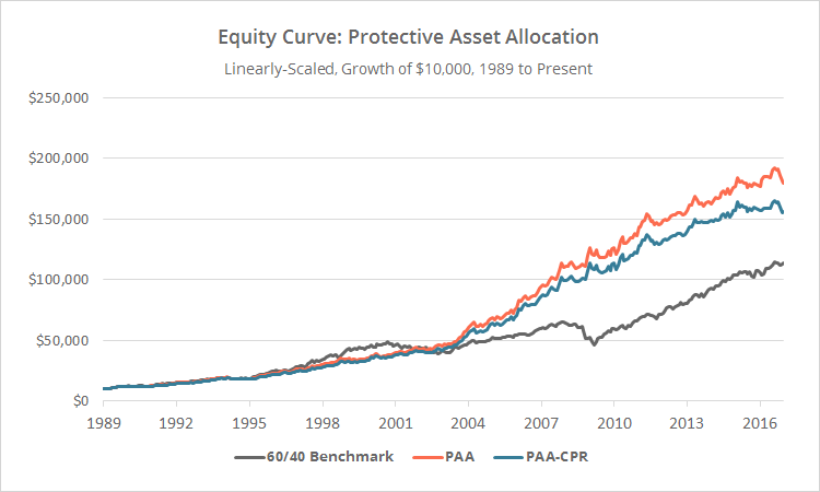
Linearly-scaled. Click for logarithmically-scaled chart.
Keller and Keuning are two of the most creative minds in tactical asset allocation, and both have been extremely supportive of our work. JW runs his own blog TrendXplorer where he talks about strategies like PAA, and I highly recommend you follow him now.
Like many of the strategies that we track, PAA is a monthly momentum trading strategy. Where PAA differs is in how aggressively it introduces a “crash protection” asset to protect the portfolio from excessive loss when just a handful of assets fail to show positive momentum.
Strategy rules tested:
I’ve tried to boil down the strategy rules to keep this description as brief as possible. For additional details, please see Keller and Keuning’s original paper.
- On the last trading day of each month (t), calculate a momentum score (MOM) for each of 12 global asset classes (see end notes for a complete list), where MOMt = [(closet / SMA(t..t-12)) – 1]. Note that the SMA is calculated based on month-end values, so t..t-12 represents the most recent 13 month-end values, including today.
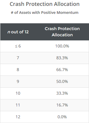
- To determine the % of the portfolio to allocate to the crash protection asset (CP) at the close, first calculate n where n equals the number of asset classes where MOM > 0. If n <= 6, then allocate the entire portfolio to the CP asset, otherwise CP % = [(12 – n) / 6]. More on the CP asset in a moment.
- If n >= 7 (or put another way, if CP % < 100%), select the 6 asset class with the highest MOM value, and allocate 1/6 of the remaining portfolio to each at the close.
- Hold positions until the final trading day of the following month. Rebalance the entire portfolio monthly, regardless of whether there is a change in position.
As previously mentioned, the strategy aggressively increases allocation to the crash protection asset based on the number of assets that fail to show positive momentum. To illustrate, the table below shows the number of assets where MOM > 0 (positive momentum), and the corresponding allocation to the crash protection asset. Note that when just 3 of 12 assets fail to show positive momentum, half of the portfolio is allocated to the CP asset.
Two variations of PAA:
This post covers two variations of Protective Asset Allocation: “PAA” and what I’m calling “PAA-CPR” (for “crash protection rotation”). Both variations allocate an average of 52% of the portfolio to the CP asset at any given time, but they differ in what assets they use as that CP asset.
In the first variation (“PAA”), the CP asset is always intermediate-term US Treasuries (IEF). This variation has been the higher returning of the two, but the devil is always in the details. This variation’s heavy reliance on IEF as a fall back asset regardless of IEF’s performance, makes the strategy particular vulnerable to an extended period of rising interest rates (read more).
In response to that, the second variation of the strategy (“PAA-CPR”) rotates the CP asset between IEF and a shorter duration instrument, depending on which has the highest MOM value. In Keller and Keuning’s original paper, this shorter-duration instrument was SHY (1-3 year US Treasuries). The problem is that, given how frequently this strategy trades, SHY might not be an appropriate asset for today’s market. Interest rates may be too low to generate enough return to overcome our assumptions about transaction costs.
To solve for that, we’ve replaced SHY with “cash” (equal to the 3-month UST rate). This reduced historical returns in our backtest, but I think is more applicable to today’s market.
Which variation is best, PAA or PAA-CPR?
Readers know that I don’t usually make these types of judgement calls. Our job is to present the data impartially and dispassionately. Having said that, if my timeframe were say the next decade, I might lean towards PAA-CPR. Some gains might be given up in the near term as this market finds its way, but there’s comfort in knowing that there’s a safety valve should we enter a new regime of rising rates.
Additional Data Dump:
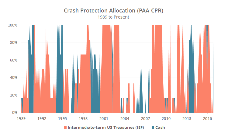
The graph below shows historical allocation to the crash protection asset for PAA-CPR (take the sum of IEF and cash for the non-CPR variation). Note the frequency with which the crash protection assets are used.
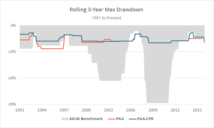
And last, as should be clear from the summary stats above, a primary advantage of this strategy historically has been in managing losses (as opposed to just generating returns). To illustrate, below I’ve plotted the rolling 3-year max drawdown for both variations versus the benchmark.
We invite you to become a member for less than $1 a day to track these and other excellent models in near real-time, or take our platform for a test drive with a free limited membership. Have questions? Learn more about what we do, check out our FAQs or contact us.
End notes:
A list of assets traded: S&P 500 (represented by SPY), Nasdaq 100 (QQQ), Russell 2000 (IWM), Europe equities (VGK), Japan equities (EWJ), emerging market equities (EEM), US real estate (VNQ), commodities (DBC), gold (GLD), US high yield bonds (HYG), US corporate bonds (LQD), long-term US Treasuries (TLT), and intermediate-term US Treasuries (IEF, crash protection asset).
There are minor differences in the assets we’ve chosen to represent each asset class versus those used by Keller and Keuning, but they are substantially similar. Also note that our test is considerably shorter than the one presented in the original paper. Generally speaking, Keller is much more liberal in creating simulated data (from prior to the launch of each ETF) than we are, allowing for a much longer backtest. That isn’t meant as a criticism; creating simulated data is a balancing act between quantity and quality of data.
