This is a test of a novel trend-following strategy from the paper Optimal Trend Following Rules in Two-State Regime-Switching Models by Valeriy Zakamulin and Javier Giner. These results aren’t as eye catching as many we track, but the paper contributes some important ideas to the study of tactical asset allocation.
Results trading the S&P 500 from 1956 follow, compared to two popular trend-following strategies. Results are net of transaction costs – see backtest assumptions. Learn more about what we do and follow 70+ asset allocation strategies like this one in near real-time.
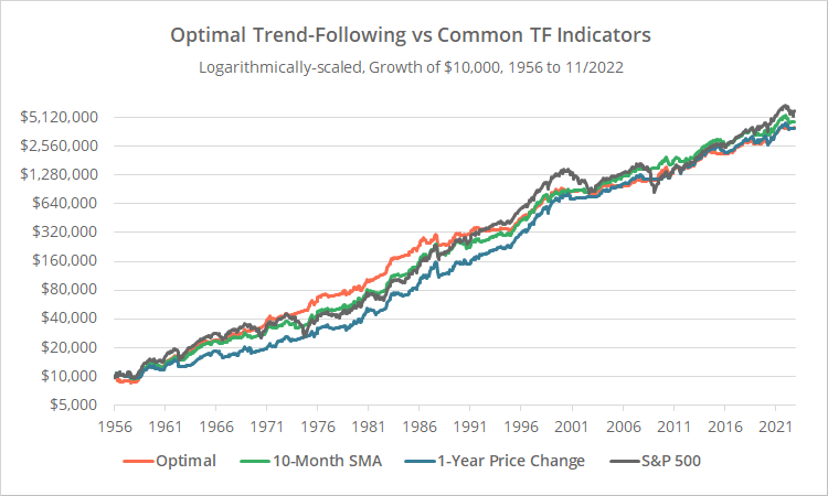
Logarithmically-scaled. Click for linearly-scaled results.
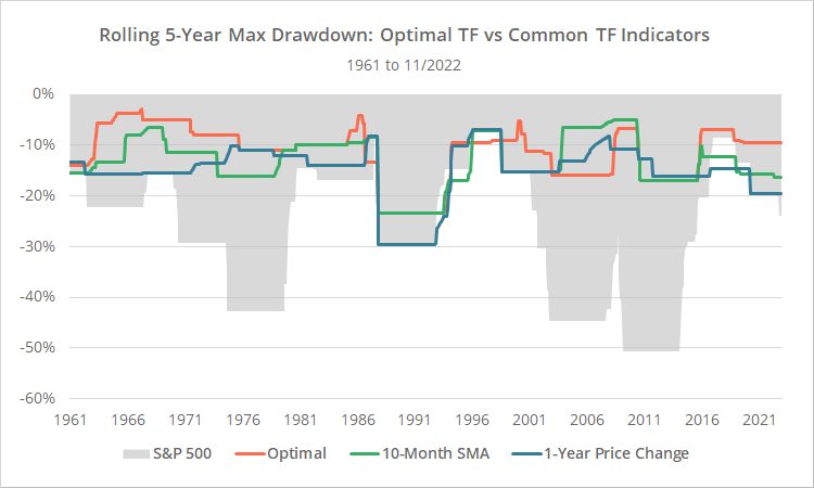
As shown below, all three trend-following strategies outperformed buy and hold on a risk-adjusted basis by better managing volatility and losses. That’s important. Short-term losses cause investors to do dumb things, usually at the worst possible time, by selling low. Providing a smooth ride helps investors control their worst impulses. The Optimal Strategy was the best performing of the bunch.
See end notes for description of the two popular trend-following strategies we’ve provided for comparison.
A novel approach to strategy design:
There are many approaches that traders use to assess whether an asset is in an uptrend or downtrend. Examples include comparing the current price to its 10-month average (ex. Meb Faber’s GTAA), comparing the current price to the price a year ago (ex. Traditional Dual Momentum), or taking a weighted average of past prices (ex. Wouter Keller’s Bold Asset Allocation).
How would one go about finding the true “optimal” trend-following indicator?
The usual approach to finding the optimal solution would be to take an asset (or basket of assets) and compare how various indicators have performed historically. Choosing the absolute top performer is likely a recipe for overfitting, so perhaps one would look for “clusters” of strong performance, or combine multiple indicators to minimize the risk of selecting just one.
Here, the authors take a unique approach.
They use what’s called a “semi-Markov switching model” (SMSM) to create a purely theoretical model of how markets behave. Characteristics of the SMSM model are based on market data from 1897 to 2020 (124 years), but there are no actual prices on which to iterate over. Rather, with their concise mathematical model in hand they can find the trend-following rules which maximize some objective function (in this case, maximizing the Sharpe Ratio).
The authors chose an SMSM because it allowed the model to be “duration dependent”. In simple terms, the model accounts for the fact that the longer the market is in a given regime (bull or bear), the higher the probability that the state will end.
Strategy rules tested:
First, understand that essentially all trend-following rules can be closely approximated using % return instead of prices. Below, the authors show how various trend-following rules weight past returns, even those like the SMA (simple moving average) that are usually based on price. The “return lag” on the X-axis represents monthly % returns based on dividend-adjusted closing prices.
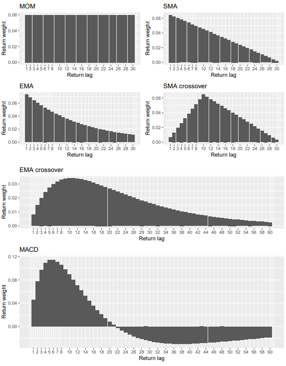
Image provided by Zakamulin and Giner.
The monthly return weighting that provides the optimal solution to the authors’ SMSM model would look as follows (orange), versus the 10-month SMA (blue).
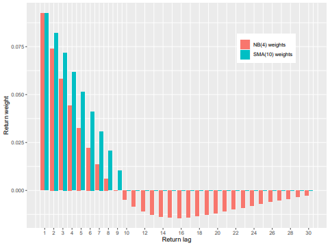
Image provided by Zakamulin and Giner.
While in the shorter-term (≤ 8 months) rising prices are a bullish indicator (and vice-versa), in the longer-term (between 10 and 30 months) they indicate the opposite; that the current state is more likely to end. This is the “duration dependence” of the SMSM model at play.
The strategy tested is as follows:
At the close on the last trading day of each month, calculate the result for the optimal trend-following indicator. If the indicator value is positive, go long the S&P 500 (represented by SPY), otherwise go to cash. Hold all positions until the close of the following month.
Our take on Optimal Trend-Following:
This is a brilliant bit of analysis by Zakamulin and Giner, and we think the concepts presented here (at the very least, the duration dependence of risk markets) is something that should be considered by other strategy authors.
Does the strategy have the same wow factor as others we track? No, but we don’t think that was the intended purpose. The authors were stripping trend-following down to its simplest form to determine the truly optimal trend-following indicator, devoid of the overfitting that is inherent when optimizing over actual past prices.
One fly in the ointment…
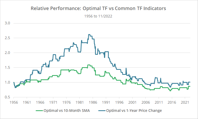
Below we’ve shown the relative performance of the Optimal Strategy versus the 10-month moving average (green) and 12-month change in price (blue) indicators. When the line is rising, the Optimal Strategy is outperforming, and vice-versa.
As previously shown, over our entire test the Optimal Strategy has outperformed other trend-following indicators, but that outperformance has ebbed over time. Note how the Optimal Strategy outperformed until the mid-1980’s, then underperformed until the mid-2000’s, and has provided essentially no added benefit since.
We wonder if the markets so fundamentally changed over the course of the very long 124-year training period, that using a shorter training period would produce a weighting more relevant to today’s market.
In any case, we appreciate the core ideas behind the Zakamulin and Giner’s analysis, and the opportunity to put those ideas to the test here. Zakamulin often posts on the Alpha Architect blog, and we highly recommend following him there.
New here?
We invite you to become a member for about a $1 a day, or take our platform for a test drive with a free membership. Put the industry’s best tactical asset allocation strategies to the test, combine them into your own custom portfolio, and follow them in real-time. Learn more about what we do.
End notes:
The two popular trend-following strategies that we’ve provided for comparison are as follows:
- 10-Month SMA: Go long the S&P 500 at the close on the last trading day of the month when the S&P 500 will close above its 10-month simple moving average (SMA), otherwise move to cash. Strategy example: Meb Faber’s GTAA.
- 1-Year Price Change: Go long the S&P 500 at the close on the last trading day of the month when the S&P 500 will close above its price 1-year ago, otherwise move to cash. Strategy example: Traditional Dual Momentum.
All prices used throughout this analysis have been adjusted for dividends.

