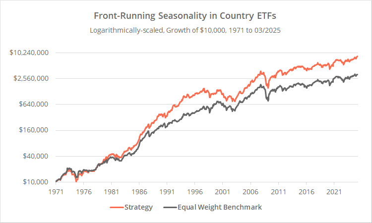
This is a test of a dynamic seasonality strategy from Quantpedia that selects from 23 individual country ETFs. We’ve extended the author’s test by 30+ years using MSCI index data.
Backtested results from 1971 follow versus an equal-weight benchmark of those 23 country ETFs (1). Learn more about what we do and follow 90+ asset allocation strategies in near real-time. Note: for reasons we discuss later, we will not be tracking this strategy on an ongoing basis.
| Summary Stats: Strategy vs Equal-Weight Benchmark 1971 to 03/2025 |
||
|---|---|---|
| Statistic | Strategy | Benchmark |
| Annual Return | 13.2% | 11.2% |
| Annual Volatility | 19.0% | 17.4% |
| Sharpe Ratio | 0.46 | 0.38 |
| Max Drawdown | -59.1% | -58.6% |
| Ulcer Perf. Index | 0.55 | 0.49 |
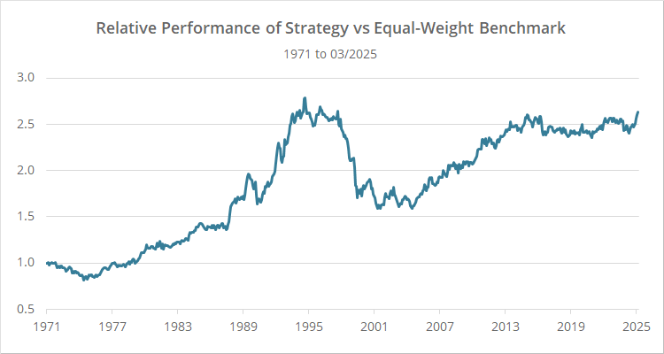
We’re also included a relative performance graph below showing the performance of this strategy relative to the equal-weight benchmark. When the line is rising, the strategy is outperforming.
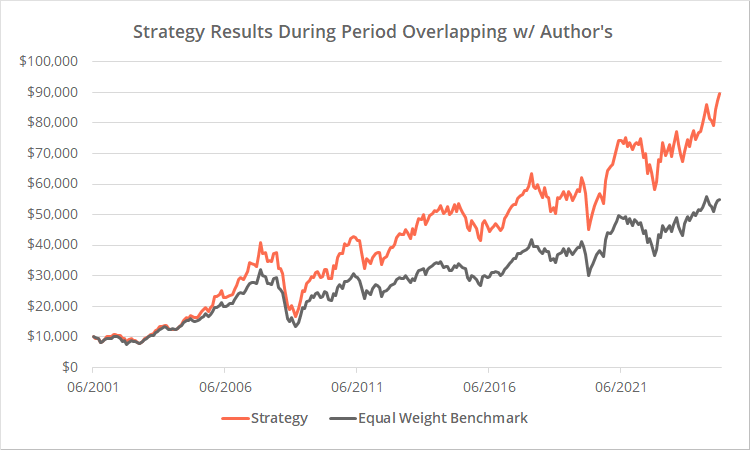
Click for a graph showing our replication over approximately the same period of time as the author’s test.
Strategy rules tested:
This strategy is part of a series from Quantpedia looking at front-running seasonality. The premise is that “traders anticipate seasonal trends and act early, shifting returns forward in time”.
-
At the close on the last trading day of the month rank all country ETFs based on their performance 10 months prior (i.e. at the end of the March, rank ETFs based on their performance in May of the previous year). (2)See Quantpedia’s original article for the list of 23 country ETFs.
- Select the top 8 ETFs and weight them as follows: rank #1-3: 18.18%, #4: 15.15%, #5: 12.12%, #6: 9.09%, #7: 6.06%, #8: 3.03%. (3)
- Hold all positions until the last trading day of the following month when the process repeats.
Strategy performance:
Our extended test results back to 1971 show that this strategy would not have been consistently effective over the long-term (although to be fair, if you ignore that period in the last half of the 1990’s, the results would appear much better).
Not adding that “front-running month” (i.e. instead forecasting month X’s return based on month X’s return last year) would have been even less effective. See the relative performance graph below.
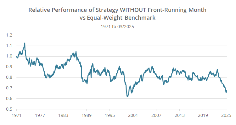
That’s a clue that there might be something to this front-running concept, but it could also just be random noise. Further testing would be required.
Based on our extended test results we will not be tracking this strategy on an ongoing basis, but we thank Quantpedia for posting a new and novel idea, and for the opportunity to put it to the test.
New here?
We invite you to become a member for about a $1 a day, or take our platform for a test drive with a free membership. Put the industry’s best Tactical Asset Allocation strategies to the test, combine them into your own custom portfolio, and follow them in real-time. Learn more about what we do.

* * *
Calculation notes:
(1) Unlike nearly all backtests on this platform, these results do not account for transaction costs.
(2) In the author’s parlance, this was the “T-11 month” (T being the month being positioned for). We’re counting T as the month the signal is actually generated, thus T-10. Same thing, different wording.
(3) In the author’s original article, it appears that they were averaging equity curves. The math of how much to allocate to each ETF in a combined strategy works out as we’ve shown it. If we were to track this strategy on an ongoing basis, we would reach out to the author for precise clarification. However, our overlapping test results match closely, and we can’t foresee any reasonable weighting scheme that would produce a significantly different result than we’ve presented, so we’ve let our assumption ride.