This is a test of two recent papers: Momentum Turning Points and Breaking Bad Trends. Learn more about what we do and follow 50+ asset allocation strategies like these in near real-time.
Successful trend-following strategies must balance the “speed” of the trading signal. If the signal is too slow, the strategy will not adapt quickly enough to changes in the actual underlying trend. If it’s too fast, the strategy will be prone to chasing every temporary fleeting change in direction.
The authors call moments when the long and short-term trend disagree “turning points”. Any trend-following strategy can succeed when the market moves in one direction, but it’s how the strategy handles these turning points that determines long-term success.
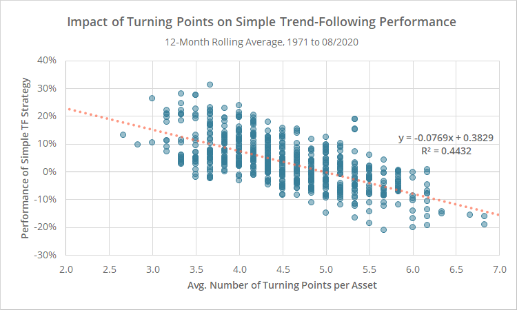
To illustrate the impact of turning points, below we’ve shown how the number of turning points over a rolling 12-month period affects the performance of a simple multi-asset trend-following strategy. Details follow after the chart.
Note how as the number of turning points (x-axis) increases, trend-following performance (y-axis) declines. Just one additional turning point per asset per year has translated to a 7.7% decline in performance for the year.
How these results were calculated:
- Monthly data, dividend-adjusted, 1971 to 08/2020.
- Define a turning point as months when the sign (+/-) of an asset’s 12-month excess return (long-term trend) differs from the sign of its 1-month excess return (short-term trend) (1)(2). One could argue that 1-month is too short to measure the short-term trend, but these results are similar when we use 2 or 3 months instead.
- The simple trend-following strategy: go long at month-end when the 12-month excess return is greater than zero, otherwise go short. Equally weight all assets in the portfolio. Hold positions until the following month.
- The authors’ results are based on a basket of 55 futures, forwards and swap contracts. At Allocate Smartly we focus on broad asset classes that can be easily traded via ETFs, so our test is based on 6 broad asset classes: US equities (represented by SPY), international equities (EFA), US Treasuries (IEF), international treasuries (BWX), commodities (DBC) and gold (GLD).
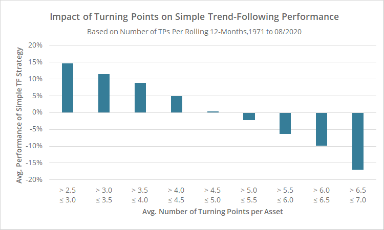
Here’s another look at the same data. Here we’ve grouped our results into buckets based on the number of turning points per year. The impact on trend-following performance is even clearer in these bucketized results.
Dealing with turning points:
We’ve shown that the frequency of turning points has a significant impact on the performance of a simple trend-following strategy. How can we better deal with these turning points to prevent this decline in performance? Put another way, how do we know when a turning point represents an actual change in the long-term trend, and when it’s just a “headfake”?
The authors propose that rather than defining a trend as simply bullish or bearish, we instead divide it four-ways based on the state of both the long and short-term trend:
- LT Trend Up, ST Trend Up: Bull
- LT Trend Up, ST Trend Down: Correction
- LT Trend Down, ST Trend Down: Bear
- LT Trend Down, ST Trend Up: Rebound
The authors then look at how the US stock market has performed following each of these four states (1). We were able to match these results precisely, so we’ve just used their charts here.
Clearly the state of the short-term trend modifies the information conveyed by the state of the long-term trend:
- Note the difference between the bull state (LT and ST trend up) and the correction state (LT up, but ST down). Both have been broadly bullish, but corrections introduce a strong negative skew, i.e. a fat left tail, i.e. a higher potential for significant loss.
- Also note the difference between the bear state (LT and ST trend down) and the rebound state (LT down, but ST up). Bear trends are bearish as one would expect, but rebounds are generally bullish.
This is just one asset class, and other assets (particularly non-risk assets like treasuries) may behave very differently during each state.
From observation to trading strategy:
The authors propose creating a unique asset allocation both for each of the four market states and for each asset.
It would be an easy task to create those optimal allocations today with the benefit of hindsight and then apply it to a historical backtest, but that would likely create an overly optimistic view of future performance. The authors instead “walk their analysis forward”.
Every 5 years, the strategy determines the optimal allocation per state per asset based on the data that was available at that time, and then uses that allocation over the next 5 years. The exact method for doing this analysis is beyond the scope of this post, but we’ve attempted to match the authors’ approach precisely, minus some not insignificant differences discussed at the end of this post. We would encourage those interested in learning more to read the source papers.
Below we’ve shown our replication of the strategy in two flavors from 1970. Results are net of transaction costs – see backtest assumptions.
The two strategies:
- The first (“Simple”) is based on the paper Momentum Turning Points, and only trades US equities (SPY).
- The second (“Portfolio”) is based on the follow up paper Breaking Bad Trends, and trades 6 asset classes: US equities (represented by SPY), international equities (EFA), US Treasuries (IEF), international treasuries (BWX), commodities (DBC) and gold (GLD). Also, unlike the analysis presented up to this point, this strategy uses the 2-month price trend (instead of 1-month) to define turning points.
The most appropriate benchmark for Simple is the S&P 500, and for Portfolio the 60/40. The benefit of both strategies (like most trend-following strategies) has been in managing risk and increasing risk-adjusted performance (ex. Sharpe, UPI). In exchange, both would have sacrificed about 1% in annual return without the introduction of leverage.
Our take on Momentum Turning Points:
As a concept, the authors are spot on. What the authors call “turning points” are the biggest challenge to trend-following/momentum investors. That should be clear to anyone who has traded this style of strategies for any length of time.
Anyone can diagnose a trend that goes in one direction in perpetuity. The difficulty lies in those moments when the market diverges from that trend. It can be difficult to determine whether that divergence is just fleeting noise or a real shift in the underlying trend. These are turning points.
Is this particular strategy the most effective approach to dealing with turning points? Probably not. Members will note that it ranks pretty poorly relative to other TAA strategies that we track.
Having said that, we applaud the attempt to quantify and respond to turning points. We also applaud the authors’ use of a walked-forward test, a useful approach for managing overfitting/hindsight bias that we wish we saw more of.
We chalk this particular strategy up to an idea that sounded good in theory but was pretty meh when actually coded up, but that doesn’t discount the importance of the topic.
New here?
We invite you to become a member for about a $1 a day, or take our platform for a test drive with a free limited membership. Put the industry’s best tactical asset allocation strategies to the test, combine them into your own custom portfolio, and follow them in near real-time. Not a DIY investor? There’s also a managed solution. Learn more about what we do.
Calculation notes:
(1) Throughout both papers, multi-month returns are not calculated as (close(t) / close(t – x) – 1) as would normally be the case. Instead, the authors use the arithmetic average of the individual monthly returns. That’s unconventional, but we’ve done the same in our replication (but not our summary stats of said replication) in order to match the authors’ results.
(2) Returns are excess of the risk-free rate. In our results, the risk-free rate is represented by the return on 13-week US T-Bills.
(3) Differences between our tests and the authors’ follow. We’ve attempted to match the spirit of the authors’ strategies, while fitting the standardized approach we take on this site: (a) long-only, (b) does not employ leverage, (c) MTP Simple calculations of a based on French data (like the paper), but trades assumed to be placed on S&P 500/SPY data, (d), MTP Simple uses rolling 5-year calculations for a, which were not introduced until second paper, (e) MTP Portfolio universe differs (see above), (f) all final positions for Portfolio that are smaller than 2% are instead placed in cash, as we assume the strategy is part of a combined model portfolio – this did not have a significant impact on results, (g) data used in calculations for a begin 07/1926 for Simple and 12/1958 for Portfolio (when possible).


