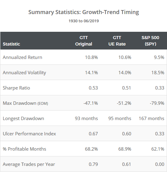
This is a test of two variations of the Growth-Trend Timing (GTT) strategy from the always thought-provoking Philosophical Economics. GTT combines trends in both price and key economic indicators to switch between US equities and cash. Like most trend-following strategies, the strength of GTT hasn’t been in generating outsized returns; it has been in maintaining returns while managing losses. Results from 1930, net of transaction costs, follow.
Read about our backtests or let AllocateSmartly help you follow these strategies in near real-time.
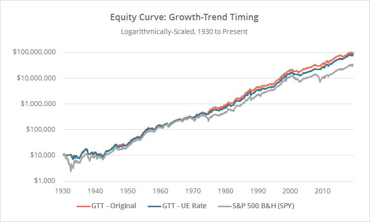
Logarithmically-scaled. Click for linearly-scaled chart.
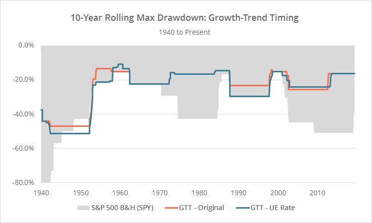
The drawdown chart is a real pile of spaghetti, so we’ve also included a rolling 10-year max drawdown version:
We covered one these GTT variations (what we’re calling “GTT-Original”) back in 2017. This updated test adds a second variation (“GTT-UE Rate”) and extends the test back to 1930. Here are links to the source material from Philosophical Economics: GTT-Original and GTT-UE Rate. The first link is a general treatise on trend-following and is highly recommended.
A note for our members: Backtests in our members area never start before 1970, because for most asset classes, reliable data doesn’t exist prior to that point. We’re able to do a much longer test here however, because GTT only trades two assets, both with a very long, reliable history: the S&P 500 and cash.
Overview:
The basic premise of the GTT strategies is that trend-following based on asset prices alone does a good job determining when to switch to defensive assets inside of recessions, but a poor job outside of recessions (see PE’s posts for evidence of that). If we have a means to judge when the economy is entering/exiting a recessionary period, we’ll know when to turn trend-following on/off.
When the strategy signals a recession, we’ll defer to trend-following to confirm, otherwise, we’ll remain long the market regardless of what price is telling us. PE reviews the efficacy of a broad range of economic indicators, and settles on three that have been the most strongly predictive of past recessions to make that determination.
Strategy rules tested:
Both variations of GTT are monthly trading strategies, changing position at the close on the last trading day of each month. We also show the results of trading on other trading days in our members area.
- The only difference between the two strategies is the economic indicators used to signal a recession. In all cases, economic indicators are calculated as of the end of the previous month. This one month lag is required due to the delay in the reporting of these numbers.
- GTT-Original: At the close on the last trading day of the month, calculate the year over year change in Real Retail and Food Services Sales (RRSFS, a measure of economic consumption) and the Industrial Production Index (INDPRO, a measure of economic production) as of the end of the previous month. If the YOY change in either indicator is negative, signal a recession.
- GTT-UE Rate: At the close on the last trading day of the month, calculate the 12-month average unemployment rate (UNRATE) as of the end of the previous month. If the previous month’s unemployment rate was higher than that 12-month average, signal a recession.
- If recession is not signaled, go long the S&P 500 (SPY) at the close.
- If recession is signaled, compare the S&P 500 (SPY) to its 10-month moving average. If it will close above the average, go long the S&P 500 (SPY) at the close, otherwise move to cash. In other words, when recession is signaled, rely on price to confirm. Note that this is the same trend-following rule used in Meb Faber’s classic GTAA.
- Hold positions until the final trading day of the following month.
Strategy performance:
Like most trend-following strategies, the strength of GTT hasn’t been in generating outsized returns; it has been in maintaining returns while managing losses.
Note the reduced max drawdown over the entire test (see rolling drawdown chart), and the increase in the Ulcer Performance Index. UPI is an important, but underutilized statistic that measures return relative to both the length and depth of drawdowns (akin to the Sharpe Ratio, but better).
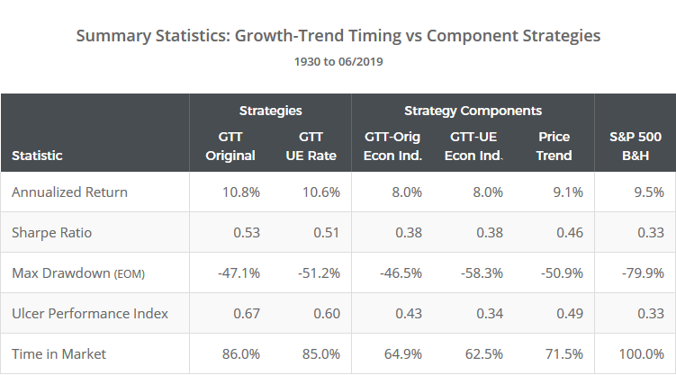
In the following table we compare each strategy to its underlying components (economic indicators and price trend) in isolation. Note the improved performance over the individual components, lending support to PE’s assertion that (a) trend-following can be improved by turning it off in non-recessionary periods, and (b) economic indicators may signal recession too early and require trend-following to confirm.
Which strategy is better?
We would say neither; knowing what we know today, they’re equally effective. The strategies agree on allocation about 96% of the time, so we’re really just talking about differences at the margin.
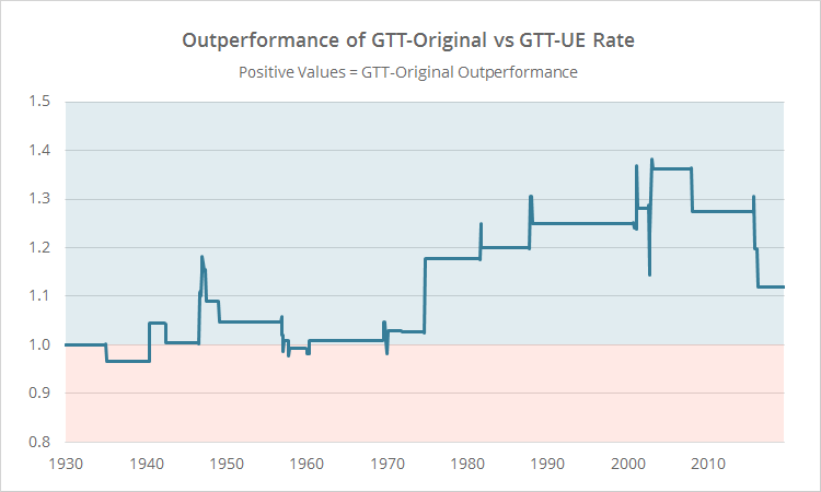
Below we’ve shown the outperformance of GTT-Original (positive values) versus GTT-UE Rate (negative values). Think of this as akin to a pairs trade between the two. Note that neither consistently outperforms the other.
What is probably better, knowing what we know today, is a combination of the two.
What’s probably even better than that, is a combination of many strategies, all using very different techniques (a challenge our site was specifically built to tackle).
A note about trading based on economic indicators:
Economic data, like that used by GTT, is often initially reported at one value and then later restated. That might happen multiple times before it finally settles on some permanent value. That could cause a change in position from what the strategy originally signaled. This is a risk inherent in trading based on economic data, and the historical results shown here are based on the economic data as it looks today.
Having said that, PE did an excellent analysis of the long-term difference between trading based on initially reported values versus restated values. In short, while it could lead to a different signal in any given month (sometimes for the worse, sometimes for the better), those differences tend to balance out over time and have little impact on long-term performance.
Our take on GTT:
We track a lot of tactical asset allocation strategies (see the list), and it’s rare that those strategies look beyond price in their trading decisions. For that reason alone, GTT has value. It would be great to see more work like this being done.
As an aside, we’ve attempted to replicate a number of popular papers that use fundamental data like this, and for reasons that escape us, we’ve repeatedly been unable to come close to the author’s optimistic results (so buyer beware). Not so here. We’ve matched PE’s numbers near perfectly (*) – a feather in their cap.
Where we find GTT lacking is that it’s not really a “total” portfolio solution – it’s a single asset class solution. It would be great to see these same concepts applied to other assets in order to build a more robust, diversified portfolio.
PE’s assertion that trend-following (and by extension, momentum) performs poorly outside of recessions has definitely held true this year. TAA as a whole has underperformed YTD after responding too quickly to market weakness in late-2018 and mid-2019, and moving to defensive assets just as the market rebounded. By “turning off” trend-following, GTT has avoided both head fakes, and performed exceptionally well.
Thank you to Philosophical Economics for all of their fine work and for the opportunity to put this model to the test. For readers interested in thorough, empirically-oriented, outside-the-box thinking on investing, we highly recommend following Philosophical Economics now.
New here?
We invite you to become a member for about a $1 a day, or take our platform for a test drive with a free limited membership. Put the industry’s best tactical asset allocation strategies to the test, combine them into your own custom portfolio, and then track them in near real-time. Have questions? Learn more about what we do, check out our FAQs or contact us.
(*) Calculation note: Even though this strategy appears pretty straight-forward, the devil is always in the details. Two of the economic series used in this test don’t extend back to 1930. We have to stitch in other related series in order to perform such a long test (see PE’s posts for details). PE was light on details about how to do that, but we’ve done our best to follow along. Small differences in our approach to stitching is a likely culprit for any discrepancies between our tests (along with our more strict backtest assumptions).
