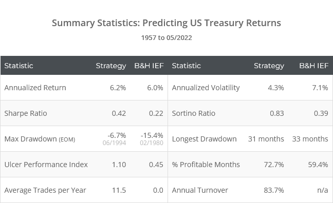
This is a test of the paper Predicting Bond Returns: 70 Years of International Evidence. The authors use an ensemble model to trade US and international treasury bonds. Over the last 60+ years the strategy would have produced long-term returns in line with buy & hold, while significantly reducing short-term volatility and drawdowns, especially during the era of rising rates.
Obviously, these results aren’t as eye catching as many of the strategies we track, but we still think the strategy could have a purpose. More on this in a bit.
Backtested results from 1957 follow. Results are net of transaction costs – see backtest assumptions. Learn about what we do and follow 60+ asset allocation strategies like this one in near real-time.

Logarithmically-scaled. Click for linearly-scaled results.
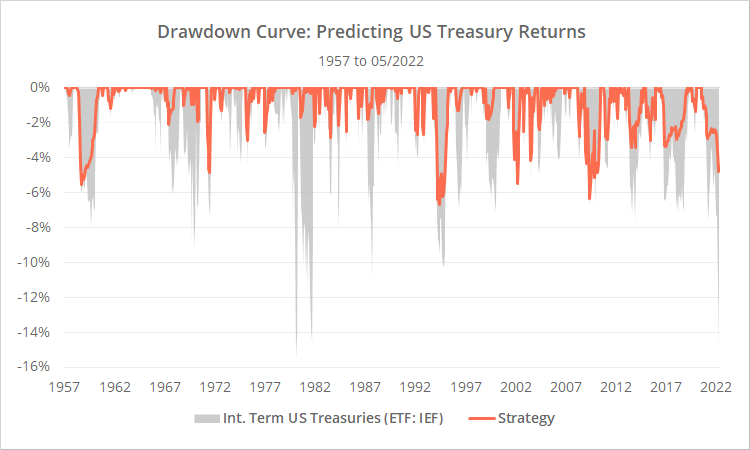
As shown in the drawdown curve below, the strategy would have consistently limited short-term drawdowns over the last 60+ years. That’s important. Short-term losses cause investors to do dumb things, usually at the worst possible time, by selling low. Providing a smooth ride helps investors control their worst impulses (and sleep better at night).
The authors applied the strategy to a global basket of both US and international treasury bonds. As a rule, we model strategies using ETFs, and that makes it impossible to replicate the strategy as it was originally designed.
We’ve opted to only apply the strategy to US Treasuries (ETF: IEF). Clearly, based on the results above, the strategy has still been an effective risk management tool in this narrower test.
Strategy rules tested:
This is an “ensemble” model, meaning it’s a mashup of four unrelated trading signals. All four signals are rooted in previous academic work and the authors do a good job addressing potential overfitting.
In short, the strategy considers four factors bullish for treasury returns: a high yield spread, a positive trend in bonds, low/negative equity returns, and low/negative commodity returns.
At the close on the last trading day of each month, generate a signal between -1 and +1 for each of the following four components:
- Yield Spread: Measure the spread between 10-year and 13-week US Treasuries. Calculate a z-score (1) based on spreads over the previous 10-years. Set a min/max z-score value of -1/+1.
- Bond Trend: Measure the return of intermediate-term US Treasuries (ETF: IEF) over the previous 12-months in excess of 3-month US Treasuries (BIL). If the excess return is > 0, the signal is +1, and if < 0, -1.
- Equity Returns: Measure the return of the S&P 500 (2) over the previous 12-months in excess of 3-month US Treasuries (BIL). Calculate a z-score based on excess return results over the previous 10-years and multiply the z-score by -1. Set a min/max z-score value of -1/+1.
- Commodity Returns: Measure the return of a diversified commodities index (DBC) (3) over the previous 12-months. Calculate a z-score based on return results over the previous 10-years and multiply the z-score by -1. Set a min/max z-score value of -1/+1.
We now have 4 signals that range between -1 and +1. To generate a final signal, we take the average of the 4 signals and perform the following: [(average + 1) / 2]. This leaves us with a final signal between 0 and 100%.
Allocate the final signal to intermediate-term US Treasuries (IEF). The remainder of the portfolio is left in cash (return on cash assumed to equal the return on 3-month US Treasuries). Hold all positions until the end of the following month.
Reduce drawdowns all the time, but only generate long-term outperformance sometimes:
As shown in the drawdown curve above, the strategy would have consistently limited short-term drawdowns over the last 60+ years. That’s important. Short-term losses cause investors to do dumb things, usually at the worst possible time, by selling low. Providing a smooth ride is important.
Over the long-term however, the strategy has essentially matched the performance of buy & hold.
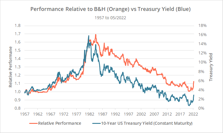
Interestingly, relative performance has been very different during eras of rising vs falling rates. In the graph below we show two series. In orange, we’ve shown the performance of the strategy relative to buy & hold. When the orange line is rising, the strategy is outperforming B&H. In blue, we’ve shown the 10-year US Treasury yield.
Note how closely the two series track each other. When rates rose prior to late 1981, the strategy strongly outperformed B&H. As rates have fallen since, the strategy has consistently underperformed.
The last 40 years have been an incredibly fortuitous time for US Treasuries, and it’s been difficult to improve on just buying and holding. If you’re of the mindset that this era of falling rates is coming to end though, then this strategy may be poised to capitalize.
In summary, this strategy would have consistently limited short-term volatility and drawdown over the entire test but has only boosted long-term returns during the era of rising rates.
So, what do we do with it?
This strategy has drastically underperformed every strategy we track on this site. That’s because (a) it’s not a total portfolio solution – it’s a single asset class solution, and (b) that single asset class just so happens to be inherently conservative.
Some degree of bond exposure will always be an important component of portfolio management, even during tough times for bonds like we find ourselves in now. Bonds help to counterbalance stocks and other risk assets, and reduce portfolio volatility.
But we’re at a unique point in history. If we are entering an era of rising rates, treasuries and other rate sensitive assets will face strong headwinds, and are mathematically guaranteed not to produce the returns investors have grown accustomed to. Investors need to adjust to that new normal.
There are multiple ways investors might do that:
- In the case of buy & hold, investors should be building portfolios that account for where rates stand today, not portfolios simply based on what’s worked in the past. See our sister site BetterBuyAndHold.com.
- In the case of tactical asset allocation (i.e. the thing we do here at Allocate Smartly), investors should be mindful of being over-exposed to rising rates. We model each strategy’s exposure to rising rates for members, and we even include it in our Portfolio Optimizer.
The strategy presented here, when used as an “overlay”, represents another option. The investor could be a little more liberal in selecting strategies with high exposure to rising rates, but then use this overlay to adjust any treasury exposure being signaled. Maybe the strategies are calling for an X% allocation to treasuries, but we reduce that based on this overlay (X% * overlay% = final%).
At the very least, we hope that the ideas presented here inspire developers to consider some of these ideas in their own strategy design.
New here?
We invite you to become a member for about a $1 a day, or take our platform for a test drive with a free membership. Put the industry’s best tactical asset allocation strategies to the test, combine them into your own custom portfolio, and follow them in real-time. Learn more about what we do.
* * *
Calculation notes:
(1) Z-score = [(x – μ) / σ]. In other words, this value minus the average of all values, divided by the standard deviation of all values.
(2) We used the S&P 500 price index (which does not account for dividends) to calculate the equity trend component, in order to stay true to the data source used by the authors. If we had instead used the dividend-adjusted S&P 500, it would have had almost no impact on these results.
(3) Geek note: Performing very distant simulations of commodity index performance is problematic because of the very different interpretations of how a commodity index should be weighted (even in today’s market), and how that interpretation has changed throughout history. Data is especially wonky prior to 1970, so we did not include commodities prior to that date. We did test using vintage CRB data prior to 1970 (which is so wonky as to be essentially unusable) and there was almost no difference in overall results, so rather than knowingly provide sketchy results, we ignored commodities altogether prior to 1970.


