This is an early preview of a new analytical tool we’ll be adding to our platform later this month. Learn more about what we do.
Broadly speaking, the goal of tactical asset allocation is to take advantage of broad market trends via trend-following and/or momentum. Those trends can be difficult to identify because of “noise”; short-term price fluctuations that confuse/distort the underlying trend.
When designing a TAA strategy, it’s important to understand whether we’ve designed to the broad trend, or whether we’ve unintentionally designed to the noise. Noise in this context is, by definition, bad information because it’s unlikely to repeat in a predictable way – it’s just randomness. Fitting our model to that randomness contributes to what’s called “overfitting”, and greatly increases the likelihood of disappointing future performance.
This new site feature is designed to measure how robust or sensitive a strategy is to noise. First we’ll discuss how we do that, then we’ll show examples of robust and sensitive strategies, and finally, we’ll talk in practical terms about what to do with this information.
How we measure “robustness to noise”:
For each of the assets that a strategy trades, we randomly add or subtract an insignificant amount of noise to each historical month (*), and then detrend the entire series so that the starting and ending values are the same. This ensures that there’s no bullish/bearish bias in our test. We run our strategy backtest and capture the stats, and then repeat the process hundreds of times.
The result is an array of possible results for the strategy, none of which is more analytical sound than any other. Let me repeat that. In terms of what they say about future performance, knowing what we know today, none of these alternative paths are any less correct than a standard backtest. Trading involves uncertainty and the performance of these alternative paths reflects that uncertainty.
This is not bootstrapping, Monte Carlo or the like. We’re not sampling from the original backtest, as that would be sampling from just one version of history. We’re changing the underlying asset data in what should be an insignificant way and looking at how the strategy responded to those changes.
See the article end notes for more details.
Example #1: A strategy that’s highly sensitive to noise
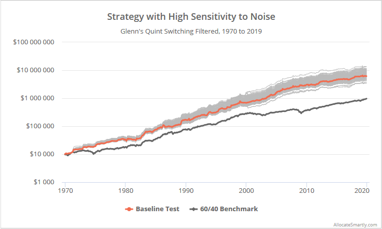
Let’s look at a strategy that’s highly sensitive to noise. This is Lewis Glenn’s Quint Switching Filtered that we covered last year. The original backtested results are in orange, versus 300 alternative paths.
For some sense of scale, we’ve also included the 60/40 benchmark in dark grey.

Logarithmically-scaled. Click for linearly-scaled chart.
Annualized returns range from 12.9% to 15.1% at the 5th and 95th percentiles respectively. View the chart in linear scale to really appreciate the dispersion. That’s quite a range of potential outcomes. Over the course of this 50 year test, that’s the difference between $1 growing to $422 and growing to $1,122 (a 2.7x increase).
It makes sense. This strategy is allocating the entire portfolio to a single asset based on a very short 3-month lookback. By TAA standards, that’s an extremely hyperactive/concentrated approach, and bound to be sensitive to small changes in asset prices.
Fortunately, the average return of our 300 noisy runs is higher than in our baseline test, so it doesn’t appear that the strategy is particularly overfit to that noise. But it does mean that an investor should expect a wide and unpredictable range of possible outcomes, and that they should take additional steps to manage that sensitivity. We’ll cover that subject in just a moment.
Example #2: A strategy that’s highly robust to noise
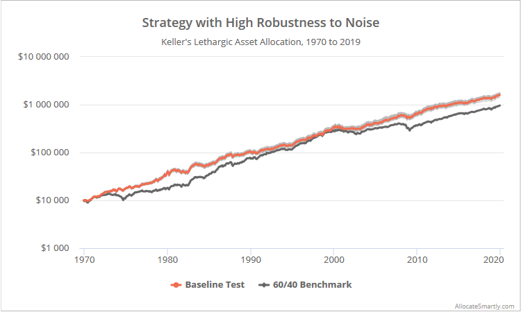
Now let’s look at a strategy that’s highly robust to noise. This is Dr. Wouter Keller’s Lethargic Asset Allocation that we covered earlier this month. The original backtested results are in orange versus 300 alternative paths, and the 60/40 benchmark in dark grey.

Logarithmically-scaled. Click for linearly-scaled chart.
Annualized returns range from 10.6% to 10.9% at the 5/95th percentiles. Nearly indistinguishable. That makes sense; LAA is mostly a buy & hold strategy, so noise is going to have less of an impact on portfolio allocation and subsequent performance.
This doesn’t necessarily mean that LAA is a “good” strategy, as there are all sorts of other factors to consider. What it does mean is that the historical result that we see for LAA is a good representation of the past. Even after we repeatedly throw a fair amount of noise at it, it generates essentially the same result.
Dealing with strategies that are sensitive to noise:
Many of the strategies that have historically been top performers are also the most sensitive to noise. That makes sense. Top performers tend to be those that make bold bets by taking concentrated positions and/or switching aggressively between offense and defense.
What then is the best approach to trading these sensitive strategies? One word: Diversification. Three approaches to accomplishing that:
- Diversification across strategies. Combining multiple strategies into a single portfolio results in a total portfolio that is more robust to noise than the constituent strategies. Our platform was specifically designed to do this.
- Diversification across trading days, i.e. tranching. Splitting the execution of monthly strategies across multiple days of the month results in a portfolio more robust to noise than putting all your eggs in a once-a-month basket. Our platform was designed to tackle this one as well.
- Better strategy design that limits “specification risk”. Read more and more. This third option is a task for strategy developers.
Outro
As always, we’re standing on the shoulders of giants here. This analysis is inspired by excellent previous work from Newfound and ReSolve, and we highly recommend following them now.
Be on the lookout for this new addition to our platform later this month. We’re still circling the drain on how to present this information in the most useful format, defining the right amount of noise to add to our tests (*), how to put this much load on our servers without our CTO strangling us, etc.
More to follow. We were just too geeked out not to share.
New here?
We invite you to become a member for about a $1 a day, or take our platform for a test drive with a free limited membership. Put the industry’s best tactical asset allocation strategies to the test, combine them into your own custom portfolio, and follow them in near real-time. Not a DIY investor? There’s also a managed solution. Learn more about what we do.
(*) We’re still defining just what the “right amount” of noise is to add to our tests. It must be done on a per asset basis, as what constitutes noise for say equities is very different than less volatile treasuries. Our current approach, a % of historical asset volatility, results in noise of, for example, approx. +/- log 0.4% on SPY and +/- log 0.2% on IEF per month.
Is that too much noise? It appears not to be. Across all strategies that we track, the average difference between the baseline backtest and the average noisy alternative is insignificant (individual strategies vary). If this were too much noise and we were “breaking” these strategies, we would expect to see broad underperformance in the noisy alternatives.
In the end, having passed the “we didn’t break the strategies” hurdle, the precise level doesn’t really matter. The absolute dispersion of the noisy alternatives is less important than the relative dispersion. In other words, strategies that are more robust at this level of noise, will likewise be more robust at twice this level or half this level, relative to other strategies. Put in even simpler terms, these statistics should not be viewed in isolation – they should be viewed relative to other strategies.
