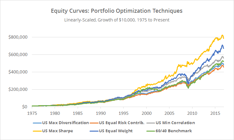
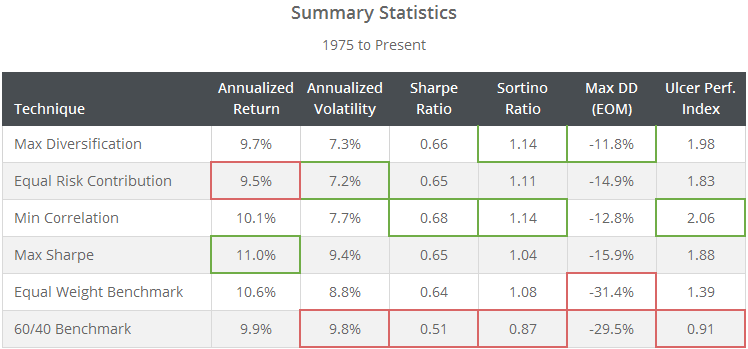
This is a test of a number of popular approaches to portfolio optimization. Each seeks to answer the question: given a universe of assets, how much should we allocate to each? We’ve intentionally made these tests as simple and fair (read: unoptimized) as possible in order to best represent each technique. Here we focus on the US market, and in a future post we’ll extend these tests to global markets. Results from 1975, net of transaction costs, follow.
Read more about our backtests or let AllocateSmartly help you follow these strategies in near real-time.

Linearly-scaled. Click for logarithmically-scaled chart.
Motivation
Most of the tactical asset allocation strategies that we track take advantage of some flavor of momentum trading, and for good reason; momentum has been the most consistently effective approach to asset allocation. At any given moment however (as we find ourselves in 2016), momentum can fall out of favor.
In my own trading, to mitigate these periods of underperformance, I overlay dynamic momentum-based TAA over a more static asset allocation. This provides a foundation for my portfolio, limits asset turnover in any given month, and can be psychologically easier to trade.
But traditional buy and hold is prone to unacceptable drawdowns, so what approach should we use for this static portion of the portfolio? Our members section includes smart approaches to buy and hold, like the All-Weather and Permanent Portfolio. The portfolio optimization techniques presented here provide another alternative.
These strategies tend to change little month to month, and have provided long-term returns in line with buy and hold without the significant drawdowns that often accompany buy and hold. While we’ve made these tests as “generic” as possible to best isolate the characteristics of each technique, one shouldn’t confuse “generic” with “ineffective”. These techniques are implicitly designed to improve on simple, naïve asset allocations.
Note from the stats above that the equal weight benchmark itself provides superior returns and lower volatility than the 60/40 benchmark, meaning that there has been value in the universe of assets itself that we’ve selected. But also note the considerable reduction in drawdown (and increase in the Ulcer Performance Index) when applying these portfolio optimization techniques, meaning that there has been added value in these optimization techniques as well.
Universe Selection
The assets that we choose to include in our portfolios is an important factor in this test. It would be easy to “improve” the historical performance of the strategies shown here by selecting an overly optimized universe of assets that’s perfectly fitted to the past, but that would say nothing about the future performance of these strategies.
In an effort to keep our test as fair as possible, we’ve selected the market’s four largest asset classes, inspired by the excellent paper The Global Multi-Asset Portfolio: equities, government bonds, non-government bonds, and real estate. These comprise the vast majority of the invested market portfolio available to individual investors.
We’ve represented each asset class as follows:
- Equities: S&P 500 (SPY). A broader ETF like VTI would be a more appropriate choice here, but the performance of the two has been similar, and SPY is commonly used throughout this site to represent US equities.
- Government bonds: Intermediate-term US Treasuries (IEF). We are intentionally ignoring shorter duration bonds to maintain portfolio volatility in the neighborhood of the 60/40 benchmark (hence the reason we didn’t use an aggregate bond ETF like AGG or BND). IEF is a nice middle ground between the remaining longer duration US Treasuries.
- Non-government bonds: US investment-grade bonds (LQD)
- Real estate: US REITs (VNQ)
We could subdivide these 4 asset classes into ever smaller groupings (for example, by dividing equities by market cap or by growth versus value), but to steer clear of any sniff of overfitting, we’ve chosen to limit our test to this simple universe.
Portfolio Optimization Techniques Tested
We’ve tested four popular portfolio optimization techniques. All except for Min Correlation require a quadratic solver to compute (we use R’s quadprog). All have been described in detail elsewhere, so for the sake of brevity, I simply list the techniques below. A quick Google search will yield a wealth of information for interested readers.
- Max Diversification
- Equal Risk Contribution (note: this is true ERC, not simple “1/volatility” risk parity)
- Min Correlation (from David Varadi)
- Max Sharpe
Assumptions made in all tests (in addition to our normal backtest assumptions):
- Portfolios are rebalanced at the close on the last trading day of every month. Practically speaking, most of these strategies could rebalance less frequently with little impact on performance, but a monthly rebalance matches most of the other strategies that we track.
- Optimization inputs are based on the previous 36 month-end values, as of that moment in time (in other words, no lookahead bias). The only exception is the Max Sharpe test – see below.
- All portfolios are long-only with no minimum or maximum allocation per asset. Total portfolio allocation will always equal 100% (i.e. no cash and no margin).
A note on the Max Sharpe strategy:
All of the techniques discussed in this post are based on asset correlation and/or volatility, except for one: Max Sharpe. Max Sharpe, also referred to as the “tangency portfolio” is different in that it also considers expected return. That’s problematic because expected return is particularly difficult to predict, and in many timeframes, is actually mean-reverting. To combat this, inspired by the excellent paper Momentum and Markowitz: A Gold Combination, each month we averaged the results of a more traditional 36-month Max Sharpe portfolio (matching the timeframe used in our other tests) with a 12-month Max Sharpe portfolio (to capture some of the momentum effect discussed in the above referenced paper). That means that, unlike the other strategies in this post, the Max Sharpe portfolio is biased by momentum.
Commentary:
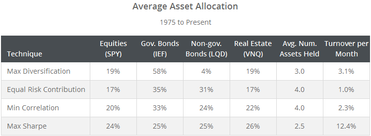
Despite similar long-term returns for most of these techniques, the assets chosen to achieve those long-term returns are sometimes very different. The table below shows each strategy’s average allocation to each asset class, as well as the average number of positions held at any given time, and the average portfolio turnover per month.
Some highlights: Note the tendency for Max Diversification to ignore non-government bonds (because they exhibit both bond-like and equity-like characteristics). Note the smaller number of assets held and higher turnover by Max Sharpe (because Max Sharpe considers expected return, which tends to be less stable than correlation/volatility). Note the similarity in average allocation between the ERC and Min Correlation techniques. And note that in all cases, exposure to gov. and non-gov. bonds is higher than the 60/40 benchmark, and I would guess, higher than most tactical asset allocators are accustomed to.
So which portfolio optimization technique is the “best”?
I don’t think that there’s a one size fits all answer.
Max Sharpe, as we’ve defined it here, is clearly the most dynamic option, but given its exposure to momentum, it might be inferior to some of the other more sophisticated momentum strategies that we track.
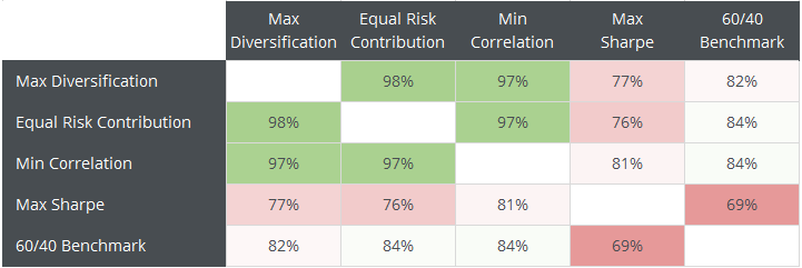
Of the remaining techniques, I personally prefer the greater diversity in allocation offered by ERC and Min Correlation. Having said that (Max Sharpe aside) the “best” is likely somewhat arbitrary given a long enough time horizon. To illustrate, below I’ve shown the monthly correlation between each strategy over the period tested. Note the high degree of correlation between Max Div, ERC and Min Corr.
Summary:
In this post we tested four popular portfolio optimization techniques applied to a universe of the four most significant US asset classes.
These techniques are not meant to be superior to the more dynamic (and often momentum-based) TAA strategies that we cover on this site, but they do have value as the foundation of a portfolio in order to limit asset turnover in any given month, and make TAA psychologically easier to trade when momentum finds itself out of favor.
We invite you to become a member for less than $1 a day to track these and other excellent models in near real-time, or take our platform for a test drive with a free limited membership. Have questions? Learn more about what we do, check out our FAQs or contact us.


