This is a test of Pragmatic Asset Allocation from Vojtko and Javorská of Quantpedia. While the strategy is “tactical” (i.e. changes allocation over time in response to market conditions), it’s also designed to ensure tax efficiency. We track many tactical strategies that have been tax efficient, but none that enforce that efficiency through explicit rules (more on this later).
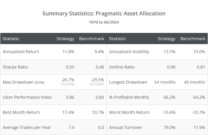
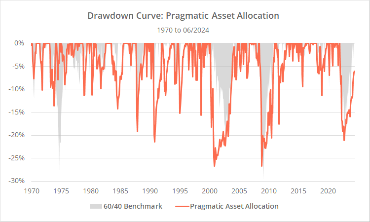
Backtested results from 1970 follow. Results are net of transaction costs – see backtest assumptions. Learn about what we do and follow 80+ asset allocation strategies like this one in near real-time.
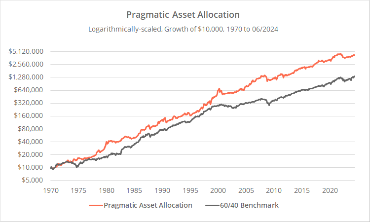
Logarithcally-scaled. Click for linearly-scaled chart.
Note: This is a rare instance where our replication is shorter than the authors’ original test. The authors started their backtest in 1928 using freely available data sources. We do not feel comfortable following suit as we have concerns about that early data and how relevant it is to today’s market.
Strategy rules tested (warning: this will be a bit of a word salad):
The strategy trades quarterly and there is a 1-month lag between generating the signal and executing trades.
The portfolio is divided into four tranches. Each tranche is independent and doesn’t affect the other tranches. The tranches trade at the close on the last trading day of months 1, 4, 7 and 10 based on a signal calculated on the last trading day of the previous month (12, 3, 6 and 9).
At the close on the last trading day of a tranche’s trading month (1, 4, 7 or 10) do the following for this tranche (and this tranche only):
- Determine if the yield curve is inverted. If the 3-month US Treasury rate exceeded the 10-year rate as of the close of the previous month (*), proceed with selecting risk assets. Otherwise, select defensive assets.
-
If selecting risk assets, measure the 12-month price change (t0 / t12 – 1) and 12-month moving average (average of t0…t11) as of the previous month for three risk asset classes: global stocks (represented by ACWI), the Nasdaq 100 (QQQ) and emerging markets (EEM).Note: All prices used throughout this test are assumed to be adjusted for dividends.
-
Sort by 12-month price change, descending. Allocate 12.5% of the portfolio (i.e. half the tranche) to each of the top two risk assets if the asset closed above its 12-month moving average as of the previous month.If less than two risk assets selected, allocate the remainder of tranche to defensive assets.
- If selecting defensive assets, measure the 12-month price change and 12-month moving average as of the previous month for 3 defensive asset classes: US int-term Treasuries (IEF), gold (GLD) and US T-Bills (BIL).
-
Sort by 12-month price change, descending. Allocate half of the remaining tranche to each of the top two defensive assets if the asset closed above its 12-month moving average, otherwise to cash.As we do throughout this platform, any funds destined for BIL are instead placed in cash.To clarify, if only 1 risk asset was selected, we still select up to 2 defensive assets here, meaning this tranche could potentially hold up to 3 assets.
At the close of trading months 1, 4, 7 and 10, for all tranches other than the current one, we also implement a “stop loss” (that is the authors’ term; this is not a conventional stop loss):
- For all assets held by the tranche, calculate the 12-month moving average as of the close of the previous month.
- If the asset closed the previous month below its 12-month moving average and the asset has already been held for more than 12 months, allocate that portion of the portfolio to cash. Remain in cash until this tranche trades again.
All trades are assumed to be executed at the close on the last trading day of the month.
Additionally, the entire portfolio (all tranches) are rebalanced monthly to their optimal “percentage of the whole”. This was a simplifying assumption on the part of the authors which we have matched, but is likely unnecessary in the real-world.
Our take on Pragmatic Asset Allocation:
We’re not going to comment on the strategy’s measure of momentum (12-month price change) or trend-following (price vs 12-month moving average), or the assets traded. This is all good and standard stuff in line with other classic TAA strategies. We have nothing smart to add.
We do want to comment on two things:
- Explicit vs de facto tax efficiency
- Inverted yield curve
Explicit vs de facto tax efficiency (only relevant if trading in a taxable account):
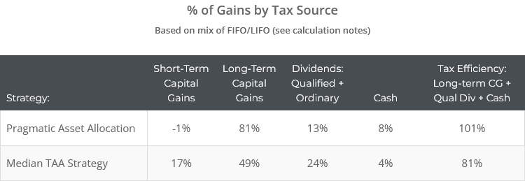
A unique characteristic of this strategy is the way it explicitly enforces tax efficiency (from a US investor’s perspective) by ensuring positions are held at least 1 year. According to our Tax Analysis, historical returns would have broken down as follows:
101% of gains would have come from something other than short-term capital gains or ordinary dividends (of course, caveats apply). Why over 100%? Because short-term trades were for a net loss.
Short-term sales were either the result of:
- The monthly rebalance which, as mentioned, is probably overkill.
- While the strategy trades on a 12 month cadence, depending on where the last day of the month this year and last year fell, positions might not exceed 365 days. Tax efficiency would be improved if the investor had executed these trades a day or so later.
De facto tax efficiency:
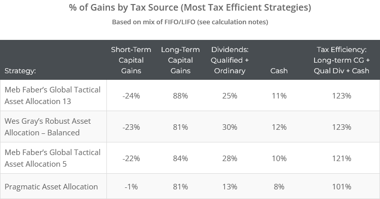
We track a number of strategies that have been even more tax efficient than Pragmatic Asset Allocation without explicit rules making them so. Three examples:
We’ve discussed previously what makes these types of strategies so tax friendly. We won’t retread that ground here. The only point we’re making is that investors don’t necessarily need explicit rules to ensure long-term tax efficiency. It can be accomplished through other aspects of strategy design.
Here’s the rub though:
While these de facto tax friendly strategies might be tax efficient in the long-term, they could be very tax inefficient in the short-term (i.e. in a particular year). There are no explicit rules preventing that. In that sense, explicit rules like those used by Pragmatic Asset Allocation might be a safer bet for investors trading in taxable accounts.
Inverted yield curve:
When the US Treasury yield curve is inverted, the strategy automatically moves the entire portfolio to defensive assets. The criteria used is the 3-month UST yield exceeding the 10-year yield.
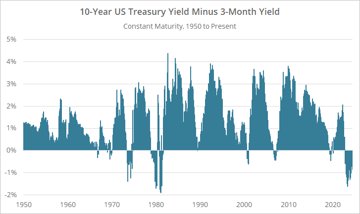
Since 1926, the yield curve has been inverted about 10% of the time. Historically, an inverted yield curve has been a leading indicator of poor future performance for risk assets. In the graph below we show the 10-year yield minus the 3-month yield. Negative values would indicate inversion and a move to defensive assets.
The yield curve has now been inverted for 20 months (based on month-end data), the longest period of inversion since at least 1926. Obviously, we haven’t seen signs of corresponding weakness in risk assets. That’s a lot of time spent on the sideline based on one single measure of market health.
Side note: the authors provide an alternate way to interpret the yield curve here.
We’re not going to comment on the fundamentals of why “this time is different” and yield curve inversion isn’t portending weakness (yet); that’s not what we do. What we will say is we would be cautious of putting so much emphasis on any single economic data point.
Asset prices don’t lie; they reflect investors’ collective valuation at that moment in time. Economic data can be much more ambiguous, and while we think it has value, we wouldn’t determine our entire portfolio’s risk posture based solely on a single data point.
We prefer the more nuanced approach to economic data taken by strategies like Growth-Trend Timing or Paul Novell’s SPY-COMP. We are wary of heavy-handed approaches to economic data taken by strategies like TrendYCMacro and Paul Choi’s Dividend and Growth Allocation.
Outro
A big thank you to Vojtko and Javorská of Quantpedia for authoring this paper. They’ve offered a unique approach to explicit tax efficiency that we haven’t seen among the 80+ strategies we track.
As always, the guys from Quantpedia were very helpful in helping us to replicate their approach precisely. We are always appreciative of authors who are so transparent and willing to expose their results to sunlight.
New here?
We invite you to become a member for about a $1 a day, or take our platform for a test drive with a free membership. Put the industry’s best Tactical Asset Allocation strategies to the test, combine them into your own custom portfolio, and follow them in real-time. Learn more about what we do.
* * *
(*) Calculation notes:
- We provide three flavors of Tax Analysis based on the share disposal method: FIFO, LIFO or “mixed”. Mixed results assume the earliest purchased shares were sold first if (a) the selling price was greater than the purchase price, and (b) the sale qualified as a long-term cap gain. Otherwise, the most recently purchased shares were sold first. In most cases, a mixed approach has been equally or more tax efficient than either FIFO or LIFO (learn more).
- We use different data series than the authors to determine yield curve inversion. The authors used the FRED series TB3MS and GS10, which are average business day values throughout the month. We use actual month-end values. This will occasionally lead to differences between our results and the authors’ in any given month, but had almost no effect over the long-term in our replication.
